Truth-tracking in a simpler case¶

Motivation for simplification¶

We are interested in aspects of truth-tracking for truth discovery. Potential questions to be answered include:

• What constraints must be placed on source trustworthiness for the truth to be discoverable?

• Which algorithms track the truth better than others?

• For a given level of source trustworthiness, how many objects are required to find the truth to within some margin of error?

Preliminary attempts to establish a framework in which to answer these questions can be found in this document. However, I think some aspects of the standard truth discovery setting are orthogonal to the core truth-tracking problem, and make analysis difficult. Namely:

• Multiple facts per object. We have considered arbitrary numbers of categorical facts for objects. This doesn’t seem like such a step up in generality from considering objects with just two facts (i.e. objects are propositional variables), but the analysis might be simpler in the propositional case.

  Dealing with more structure in the facts might be best left to future work. Some existing papers already look specifically at generalising TD to handle different kinds of facts, e.g. [LLG+16] introduces a general framework for heterogeneous data which just requires a distance metric for each data type.

• Partial claims. This adds additional complexity since we need to consider how ‘full’ the dataset is. Intuitively it seems harder to track the truth if each source makes few claims. But this seems like a separate problem which is not essential for truth-tracking.

  Dealing with partial information in social choice settings seems like its own research area, e.g. Chapter 10 of [BCE+16].

Proposed setting¶

I propose a simpler setting very similar to judgement aggregation and work around Condorcet’s Jury Theorem (the original truth-tracking result). This might allow easier progress while still retaining the relevant TD features:

• Propositional objects. Consider propositional atoms \(A_n = \{a_1,\ldots,a_n\}\).

• Full information. Each source submits a valuation over \(A_n\) (i.e. gives a truth value for each atom)

• Simple probabilistic model. A state of the world is a pair \(\theta=(w^*, v^*)\), where

  • \(w^*=(p_1,\ldots,p_m) \in [0,1]^m\) are the (probabilistic) reliability levels of each of \(m\) sources

  • \(v^*\) is a valuation over \(A_n\)

  A state \(\theta\) then defines a probability distribution over TD networks: source \(j\) makes a correct claim on \(a_i\) with probability \(p_j\).

• Operators. An operator \(T\) maps the inputs of \(m\) sources over \(n\) atoms to a pair \((w, v)\), i.e. a potential state of the world

• Truth-tracking. We can look at \(\prob{v_N^T = v^* \mid \theta}\) for the probability that the valuation \(v_N^T\) given by \(T\) on a random network \(N\) matches the true valuation according to \(\theta\)

• Trust-tracking. Can look at \(E_{N \mid \theta}\|w_N^T - w^*\|\) for the expected difference between estimated and true source weights

Note that one of the main problems of judgement aggregation – ensuring consistency of the aggregated judgement – is avoided since the formulas on which sources report and logically independent.

Related work¶

There seems to be a huge body of literature (esp. 80s - 90s?) around things like Condorcet’s Jury Theorem and its generalisations.

TODO: read these papers in full.

• Optimal Decision Rules in Uncertain Dichotomous Choice Situations (Nitzan and Paroush, 1982)

  Proves that a ‘weighted majority rule’ is optimal for finding the truth when there is just a single object to be decided on.

• Thirteen Theorems in Search of the Truth (Grofman et. al., 1983)

  Gives an overview of truth-tracking-like results from the 80s in the case of a single object. Most important is the classic jury theorem: if all the \(p_i\)s are constant and greater than 0.5, then majority rule finds the truth with probability 1 in the limit as the number of sources goes to infinity. Some other results:

  • Necessary and sufficient conditions on the \(p_i\)s (not necessarily constant) which ensure majority is correct with probability greater than 0.5. In particular, for a small number of sources the mean reliability can be less than 0.5 but majority accuracy greater than 0.5 (and vice versa!). But this affect diminishes as \(m \to \infty\).

  • ‘Generalised Condorcet Jury Theorem’: deal with truth-finding in the limit. Same as Condorcet Jury theorem but constant reliability \(p\) is replaced with mean reliability of the \(p_i\).

• Distilling the wisdom of crowds: weighted aggregation of decisions on multiple issues (Baharad et. al., 2011)

  Considers the proposed setting above (pretty much), and introduces a maximum likelihood estimation algorithm for finding the \(p_i\)s.

• Beyond Condorcet: Optimal aggregation rules using voting records (Baharad et. al., 2012)

  A lot of overlap with the above paper…

Research directions¶

Based on a brief read of some papers in the area, the following might be areas in which to do something new:

• Look beyond the majority rule. A lot of papers seem to have the case \(p_i > 0.5\) in mind, so the focus is on the majority rule. But in TD we expressly don’t want to use majority (which is the same as plurality in the 2-alternative case). How do other methods (mainstream TD or otherwise) perform wrt truth-tracking?

  Related to this, we could look to find the situations in which the truth can be found by some operator (c.f. Truth-Tracking by Belief Revision? [BGS19]), not just found by majority. Here ‘situations’ means some properties of the reliability distribution \(w^*\) (e.g. the mean or variance of reliability levels?).

• Simultaneous trust and truth tracking. The paper Distilling the wisdom of crowds… seems to look at finding the reliability weights \(p_i\) using MLE in order to estimate the true status of each proposition. If there is some theoretical guarantee that their methods find both \(w^*\) and \(v^*\) (using the above notation) in an optimal way, does this mean truth discovery has been solved? If not, there might be something to work on.

  For example, is it the case than an operator which tracks the reliability weights well will also track the truth well? Or is there a trade-off?

• Sample complexity (using terminology from [CPS16]). Rather than look at truth-tracking in the limit, ask the following question: for reliability weights \(w^*\) for a fixed number of sources, how many objects are required to find the truth (either on the whole or wrt a particular proposition) with probability \(1 - \epsilon\)? This would allow more fine-grained comparison between operators; even if two operators both find the truth in the limit as we have more and more information, one might get there sooner than the other.

Reading list¶

• Aggregating Binary Judgments Ranked By Accuracy (2020) [HKP+20]

• Optimizing group judgmental accuracy in the presence of interdependencies (1984)

• The Condorcet Jury Theorem, Free Speech, and Correlated Votes (1992)

• Test Theory Without an Answer Key (1998)

• A Nonasymptotic Condorcet Jury Theorem (2000). Contains a lot of useful references in the introduction.

• Who moderates the moderators?: crowdsourcing abuse detection in user-generated content (2014)

• Voting with Limited Information and Many Alternatives (2014)

Probability references¶

• Lecture notes from Elias Koutsoupias. Lectures 7 - 12 introduce Chernoff bounds, Hoeffding’s inequality and others, which might be helpful.

• Chapter 20 of Mathematics for Computer Science: ‘Deviation from the mean’

• ‘Concentration inequalities’ on Wikipedia.

Musings¶

Informal collection of thoughts on different aspects relating to the above research goals. Notation may not be final.

Optimal aggregation rules when the \(p_i\) are known¶

This section begins with a retelling of (some of) the work of Nitzan and Paroush from 1982 [NP82] with some steps of the proofs written in more detail, and using notation that makes more sense to me. I then attempt to study the sample complexity of the optimal aggregation rule in this setting.

The setting is similar to above, but here we explicitly model the correct judgement (0 or 1) by a random variable \(Z\). Write \(\prob{Z = 1} = \alpha\); we will assume \(\alpha \in (0, 1)\). Let \(X_i\) represent the judgement of source \(i\) (for \(1 \le i \le n\)). We assume the \(X_i\) are conditionally independent given \(Z\), with

\[\begin{aligned} \prob{X_i = 1 \mid Z = 1} &= p_i \\ \prob{X_i = 1 \mid Z = 0} &= 1 - p_i \end{aligned} \]

where \(p_i \in (0, 1)\) is the reliability of source \(i\). Note an important assumption at this stage: sources are correct with the same probability when \(Z=1\) or \(Z=0\). That is, the reliability of sources does not depend on the true judgement.

Next, write \(Y_i = \indicator{X_i = Z}\), 1 so that \(Y_i = 1\) iff source \(i\) is correct. It is easy to check that (due the above assumption) \(Y_i\) takes value 1 with probability \(p_i\), and each \(Y_i\) is independent of \(Z\) (and of the other \(Y_j\)).

An aggregation rule is a function \(f: \{0,1\}^n \to \{0,1\}\). For such a function, let \(Y_f = \indicator{f(X_1,\ldots,X_n) = Z}\), i.e. \(Y_f = 1\) iff the aggregated judgement (according to \(f\)) is correct.

Definition 1

\(f\) is optimal if \(\prob{Y_f = 1} \ge \prob{Y_{f'} = 1}\) for all aggregation rules \(f'\).

That is, \(f\) is optimal if there is no other rule with strictly higher probability of being correct. Nitzan and Paroush showed that the following weighted aggregation rule is optimal.

Proposition 2 ([NP82])

Write \(w_i = \log\frac{p_i}{1-p_i}\), \(W = \sum_{i=1}^{n}{w_i}\) and \(\gamma = \onehalf\log\frac{\alpha}{1-\alpha}\). Define \(\hat{f}\) by

\[\hat{f}(x_1,\ldots,x_n) = \indicator{ \gamma + \sum_{i=1}^{n}{w_i x_i} \ge \onehalf W }\]

Then \(\hat{f}\) is optimal.

Proof.

Let \(f\) be an arbitrary aggregation function. Write \(\vec{X} = (X_1,\ldots,X_n)\) and \(\vec{Y} = (Y_1,\ldots,Y_n)\). We have

\[\begin{aligned} \prob{Y_f = 1} &= \alpha \cdot \prob{Y_f = 1 \mid Z = 1} + (1 - \alpha) \cdot \prob{Y_f = 1 \mid Z = 0} \\ &= \alpha \cdot \prob{f(\vec{X}) = 1 \mid Z = 1} \\ & \quad + (1 - \alpha) \cdot \prob{f(\vec{X}) = 0 \mid Z = 0} \end{aligned} \]

Note that if \(Z=1\) we have \(X_i = Y_i\), and if \(Z=0\) we have \(X_i = 1 - Y_i\). Using this fact together with the independence of the \(Y_i\) from \(Z\), we have

\[\begin{aligned} \prob{f(\vec{X}) = 1 \mid Z = 1} &= \prob{f(\vec{Y}) = 1 \mid Z = 1} \\ &= \prob{\vec{Y} \in f^{-1}(1) \mid Z = 1} \\ &= \prob{\vec{Y} \in f^{-1}(1)} \\ \end{aligned} \]

and similarly

\[\begin{aligned} \prob{f(\vec{X}) = 0 \mid Z = 0} &= \prob{f(1 - \vec{Y}) = 0 \mid Z = 0} \\ &= \prob{1 - \vec{Y} \in f^{-1}(0)} \end{aligned} \]

Hence

\[\begin{aligned} \prob{Y_f = 1} &= \alpha \cdot \prob{\vec{Y} \in f^{-1}(1)} + (1 - \alpha) \cdot \prob{1 - \vec{Y} \in f^{-1}(0)} \\ &= \alpha \sum_{\vec{y} \in f^{-1}(1)}{\prob{\vec{Y} = \vec{y}}} + (1 - \alpha) \sum_{\vec{y} \in f^{-1}(0)}{\prob{\vec{Y} = 1 - \vec{y}}} \\ &= \sum_{\vec{y} \in \{0,1\}^n}{ \left( \alpha f(\vec{y}) \prob{\vec{Y} = \vec{y}} + (1 - \alpha) (1 - f(\vec{y})) \prob{\vec{Y} = 1 - \vec{y}} \right) } \\ &= \sum_{\vec{y} \in \{0,1\}^n}{ \left( f(\vec{y}) A(\vec{y}) + (1 - f(\vec{y})) B(\vec{y}) \right) } \end{aligned}\tag{2} \]

where \(A(\vec{y}) = \alpha \cdot \prob{\vec{Y} = \vec{y}}\) and \(B(\vec{y}) = (1 - \alpha) \cdot \prob{\vec{Y} = 1 - \vec{y}}\). Note that since \(f(\vec{y}) \in \{0, 1\}\), exactly one of the terms in the summand is non-zero, and thus

\[\prob{Y_f = 1} \le \sum_{\vec{y} \in \{0,1\}^n}{ \max\left\{ A(\vec{y}), B(\vec{y}) \right\} } \tag{3}\]

We will show that \(\hat{f}\) achieves this upper bound and is therefore optimal. Indeed, let \(\vec{y} = (y_1,\ldots,y_n) \in \{0,1\}^n\). Due to the independence of the \(Y_i\) we have

\[\begin{aligned} \prob{\vec{Y} = \vec{y}} &= \prod_{i=1}^{n}{\prob{Y_i = y_i}} \\ &= \prod_{i\ :\ y_i = 1}{p_i} \cdot \prod_{i\ :\ y_i = 0}{(1-p_i)} \end{aligned}\]

and similarly

\[\begin{aligned} \prob{\vec{Y} = 1 - \vec{y}} &= \prod_{i\ :\ 1 - y_i = 1}{p_i} \cdot \prod_{i\ :\ 1 - y_i = 0}{(1-p_i)} \\ &= \prod_{i\ :\ y_i = 0}{p_i} \cdot \prod_{i\ :\ y_i = 1}{(1-p_i)} \end{aligned}\]

This means

\[\begin{aligned} A(\vec{y}) &\ge B(\vec{y}) \\ &\iff \alpha \cdot \prob{\vec{Y} = \vec{y}} \ge (1 - \alpha) \cdot \prob{\vec{Y} = 1 - \vec{y}} \\ &\iff \alpha \prod_{i\ :\ y_i = 1}{p_i} \cdot \prod_{i\ :\ y_i = 0}{(1-p_i)} \ge (1 - \alpha) \prod_{i\ :\ y_i = 0}{p_i} \cdot \prod_{i\ :\ y_i = 1}{(1-p_i)} \\ &\iff \frac{\alpha}{1 - \alpha} \prod_{i\ :\ y_i = 1}{\frac{p_i}{1 - p_i}} \ge \prod_{i\ :\ y_i = 0}{\frac{p_i}{1 - p_i}} \end{aligned}\]

Taking the logarithm of both sides, we get

\[\begin{aligned} A(\vec{y}) &\ge B(\vec{y}) \\ &\iff \log{\frac{\alpha}{1 - \alpha}} + \sum_{i\ :\ y_i = 1}{w_i} \ge \sum_{i\ :\ y_i = 0}{w_i} \\ &\iff 2\gamma + \sum_{i=1}^{n}{w_i y_i} \ge \sum_{i=1}^{n}{w_i (1 - y_i)} \\ &\iff 2\gamma + \sum_{i=1}^{n}{w_i y_i} \ge W - \sum_{i=1}^{n}{w_i y_i} \\ &\iff 2\gamma + 2\sum_{i=1}^{n}{w_i y_i} \ge W \\ &\iff \gamma + \sum_{i=1}^{n}{w_i y_i} \ge \onehalf W \\ &\iff \hat{f}(\vec{y}) = 1 \end{aligned}\]

It follows that \(f(\vec{y})A(\vec{y}) + (1 - f(\vec{y}))B(\vec{y}) = \max\{A(\vec{y}), B(\vec{y})\}\). Returning to \((2)\) we see that \(\prob{Y_{\hat{f}} = 1}\) achieves the upper bound from \((3)\), and we are done.

Here the weights \(w_i\) are the log odds of the reliability levels \(p_i\). \(\hat{f}\) outputs \(1\) if the sum of \(\gamma\) and the weights of sources voting for \(1\) (i.e. those \(i\) for whom \(x_i = i\)) exceeds half of the total weight. Note that \(\gamma > 0\) if \(\alpha > \onehalf\) and \(\gamma < 0\) if \(\alpha < \onehalf\). One can interpret this as the \(1\)-voters receiving a boost of \(\gamma\) when we already believe \(Z=1\) to be more likely than \(Z = 0\), and the \(0\)-voters receiving the boost in the opposite case.

In the special case where \(\alpha = \onehalf\) (i.e. when we have no prior information about \(Z\)), \(\gamma = 0\) and \(\hat{f}\) becomes a weighted majority rule.

Sample complexity¶

To keep things simple, consider the case \(\alpha = \onehalf\) only. The following can be obtained by Hoeffding’s inequality in a similar way to Proposition 1, although it is not clear how useful the result is…

Proposition 3

Let \(\epsilon > 0\). Write \(\lambda_i = |w_i| \cdot{|p_i-\onehalf|}\) and \(\bar{\lambda} = \frac{1}{n}\sum_{i=1}^{n}{\lambda_i}\). Suppose there is at least one \(i\) with \(p_i \ne \onehalf\), and

\[n \ge \frac{\|\vec{w}\|}{\bar{\lambda}} \sqrt{\onehalf \log\frac{1}{\epsilon}} \tag{4}\]

where \(\vec{w} = (w_1, \ldots, w_n)\) and \(\|\cdot\|\) is the Euclidean norm.

Then the weighted aggregation rule \(\hat{f}\) is correct with probability at least \(1 - \epsilon\).

Proof.

Since the bound is not too impressive or useful, I will only sketch the steps to proving it.

1. Define random variables \(\tilde{X}_i\) by \(\tilde{X}_i = X_i\) if \(p_i \ge \onehalf\) and \(\tilde{X}_i = 1 - X_i\) if \(p < \onehalf\). Define \(\tilde{Y}_i = \indicator{\tilde{X}_i = Z}\) and observe that \(\tilde{Y}_i\) is equal to either \(Y_i\) or \(1 - Y_i\) according to whether \(p_i \ge \onehalf\) or \(p_i < \onehalf\).

   Intuitively, \(\tilde{X}_i\) is the judgement given by source \(i\), but flipped if source \(i\) is strictly worse than random chance. We have \(\prob{\tilde{Y}_i = 1} = \max\{p_i, 1 - p_i\} \ge \onehalf\) for all \(i\).

2. Observe that \(\prob{Y_{\hat{f}} = 1} \ge \prob{\sum_{i=1}^{n}{w_i Y_i} > \onehalf W}\).

3. Split the sum up according to those \(i\) with \(p_i \ge \onehalf\) and those with \(p_i < \onehalf\) to show that

   \[\sum_{i=1}^{n}{w_i Y_i} > \onehalf W \iff \sum_{i=1}^{n}{|w_i| \tilde{Y}_i} > \onehalf \sum_{i=1}^{n}{|w_i|}\]

4. Consider the following variant of Hoeffding’s inequality: if \(Q_1,\ldots,Q_n\) are independent with \(\prob{Q_i \in [a_i, b_i]} = 1\) for each \(i\) and \(Q = \sum_{i=1}^{n}{Q_i}\), then

   \[\prob{Q - \expect{Q} \le -t} \le \exp\left(-\frac{2t^2}{\sum_{i=1}^{n}{(b_i - a_i)^2}}\right)\]

5. Apply with \(Q_i = |w_i| \tilde{Y}_i\), taking \(a_i = 0\) and \(b_i = |w_i|\), to get

   \[\begin{aligned} \prob{\hat{f} \text{ is incorrect }} &\le \prob{ Q - \expect{Q} \le -\left(\expect{Q} - \onehalf\sum_{i=1}^{n}{|w_i|}\right) } \\ &= \prob{ Q - \expect{Q} \le - \left( \sum_{i=1}^{n}{ |w_i|( \underbrace{\expect{\tilde{Y}_i} - \onehalf}_{ |p_i - \onehalf| } ) } \right) } \\ &= \prob{Q - \expect{Q} \le - \sum_{i=1}^{n}{\lambda_i}} \\ &= \prob{Q - \expect{Q} \le - n \bar{\lambda}} \\ &\le \exp\left( -\frac{2(n\bar{\lambda})^2}{\sum_{i=1}^{n}{|w_i|^2}} \right) \\ &= \exp\left( -\frac{2(n\bar{\lambda})^2}{\|\vec{w}\|^2} \right) \\ &\le \epsilon \end{aligned}\]

   where the last step follows from \((4)\).

Remarks.

• The dependence on \(\epsilon\) has been taken under a square root compared to Proposition 1.

• The result holds regardless of the mean reliability levels \(p_i\). This is obvious, since when the \(p_i\) are known we can always flip the judgements of those \(i\) with \(p_i < \onehalf\) to get better than random chance accuracy. Indeed, the important quantity is \(|p_i - \onehalf|\): the distance of \(p_i\) from random chance.

• It is harder to understand the RHS independently of \(n\) here, which certainly makes this less appealing as a sample complexity bound. \(\bar{\lambda}\) is a kind of average ‘weighted reliability’ (so perhaps comparable to \(\bar{p}\) in Proposition 1?). But \(\|\vec{w}\|\) is the overall size of the weights, which does change with \(n\) (e.g. adding a new source causes \(\|\vec{w}\|\) to increase).

• I don’t know what happens to the leading term \(\|\vec{w}\| / \bar{\lambda}\) in general as the \(p_i\) get larger. On the on hand, each \(\lambda_i\) goes quickly to \(+\infty\) as \(p_i\) goes away from \(\onehalf\) (see Figure 1), but \(\|\vec{w}\|\) also increases with the \(p_i\).

  Ideally we want \(\|\vec{w}\| / \bar{\lambda}\) to be small, since this gives a lower sample complexity in \((4)\). Figure 2 shows how this quantity changes w.r.t \(p_1\) when \(p_2\) is fixed, in the case \(n=2\). This is promising, since we see a decrease as \(p_1\) gets more informative (i.e. away from \(\onehalf\)), until \(p_1\) gets very close to 0 or 1. 2 The weights are undefined at these points, and it seems that \(\|\vec{w}\| / \bar{\lambda}\) goes to \(+\infty\). If true this makes the bound in \((4)\) useless as \(p_1 \to 1\).

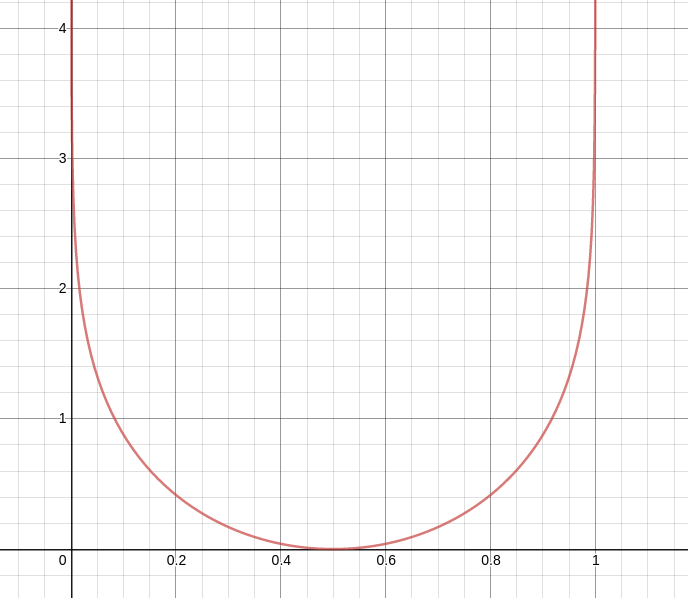
Figure 1: \(\lambda(p) = \left|\log\frac{p}{1-p}\right| \cdot{|p-\onehalf|}\)¶

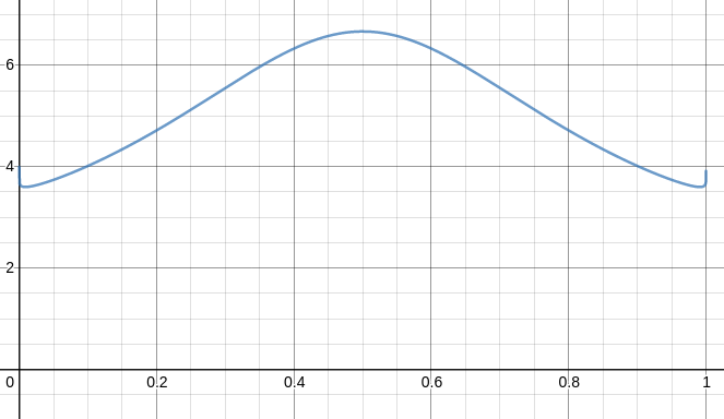
Figure 2: Plot showing \(\|\vec{w}\| / \bar{\lambda}\) for \(n = 2\). Here the horizontal axis is \(p_1\), and \(p_2\) is fixed at 0.8.¶

---

1

Here \(\indicator{p} = 1\) if \(p\) is true and 0 if \(p\) is false.

2

Manualy zooming in on the graph of Figure 2 shows that \(\|\vec{w}\| / \bar{\lambda}\) start to increase around \(p_1 < 0.001\) and \(p_1 > 0.991\).