Misc papers
How to trust a few among many (2017)
(Anthony Etuk and Timothy Norman and Murat Sensoy and Mudhakar Srivatsa)
Summary:
Core idea: decision-making under resource constraints: cannot gather reports from loads of sources (e.g. due to cost or time constraints)
Similar sources – who are likely to provide similar opinions – can be grouped together
Grouping can be done along various features: e.g. expertise, geographic location, others…
Interesting that it explicitly represents features of sources; they are not just abstract entities like in many TD approaches
This minimises redundant sampling (sample sources from different groups rather than two from the same group) and accounts for dependence between sources (‘herd mentality’, copying etc)
Their framework can inform an agent on whom to ask for an opinion on a given topic
Decision-making context seems to be environmental issues – e.g. weather at a particular location, river water depth, number of casualties after an accident 1
Framework:
Trust in Information through Diversity (TIDY)
Summary of framework:
Learns similarity metric on sources from historic reports
Sources clustered basic on similarity
Sampling strategy uses clusters to decide from whom to obtain reports
Reports are fused to provide an estimate of world state
Preliminaries:
\(\Theta\) represents possible values of a variable of interest
\(T\) is a set of timestamps
\(\theta^t \in \Theta\) is the true value at time \(t \in T\)
The set of sources is \(\mathcal{N}=\{1,\ldots,n\}\)
\(F= \{f_1,\ldots,f_d\}\) is a set of features, which are observable properties of sources. Each feature \(f_i\) has a domain \(D_i\). A source has an associated feature vector \(V_x \in \hat{D_1} \times \ldots \times \hat{D_d}\), where \(\hat{D_i} = D_i \cup \{null\}\). Here \(null\) denotes that the feature is not applicable for a particular source.
The report from source \(x\) at time \(t\) is denoted by \(o_x^t \in \Theta \cup \{\perp\}\), where \(\perp\) denotes the absence of a provided value. The set \(O_x^T = \{o_x^t : t \in T\}\) denotes all reports from source \(x\)
A diversity structure is a partition \(\mathcal{DS} = \{G_1,\ldots,G_K\}\) of \(\mathcal{N}\)
Source agreement:
\(\Pi_{agr}\) is an ordered set of agreement values (e.g. \(\Pi_{agr} = \{0, 1\}\))
A report agreement function \(v_{agr}\) gives the agreement level \(v_{agr}(t, o_x^t, o_y^t) \in \Pi_{agr} \cup \{\perp\}\) between the reports provided by \(x\) and \(y\) at time \(t\)
A source agreement function \(\sigma\) given the agreement level \(\sigma(x, y, v_{agr}) \in \R\) between two sources (with respect to \(v_{agr}\))
A function \(\text{revise\_metric}\) computes a metric \(\text{revise\_metric}(\sigma) : \mathcal{N}^2 \to \R\) on sources based on agreement of sources
Trust assessment:
A function \(v_{tru}\) gives a trust assessment \(v_{tru}(t, o_x^t, \theta) \in \Pi_{tru} \cup \{\perp\}\) of the value provided by \(x\) against the known ground truth \(\theta\)
\(\tau(x, v_{tru}) \in \R\) is the trustworthiness of source \(x\) with respect to \(v_{tru}\)
Sampling:
Sampling sources is not free: a cost function \(\text{cost}: 2^\mathcal{N} \to \R\) gives the cost for a subset of sources
Aim to select a subset \(N \subseteq \mathcal{N}\) to maximise the expected accuracy of information (with respect to the truth) whilst minimising cost
Instantiation of the framework:
Specific examples for \(v_{agr}\) and \(v_{tru}\)
Discusses a decision tree-based method for learning source distance metric on sources based on their features (training data includes features of pairs of sources and their agreement level \(\sigma(x, y)\))
Hierarchical clustering using the learned distance metric to form the ‘diversity structure’ (partition of sources)
Discusses methods for choosing which sources to sample given a fixed budget
Fusion method (roughly) averages reports from sources in the same cluster; weights cluster averages by cluster trustworthiness; combines weighted averages to produce final prediction
Experimental analysis
Truth approximation, belief merging, and peer disagreement (2014)
(Cevolani, Gustavo)
Summary:
Looks at how and whether belief merging can lead to a position closer to the truth than the individual agents’ inputs.
Highlights the principle that disagreement between agents may be a benefit in seeking the truth, since it may lead to discussion and rational argument.
Idea is that agents are “epistemic peers”: they trust each other and are all reliable regarding the matter at hand. [E.g. think of a bunch of expert scientists having discussion]. They wish to merge their beliefs to a collective decision; the goal is to take everyone’s viewpoint into account (including the disagreements between agents) and come to a final position closer to the truth than each agent’s individual position.
If the above is achieved, the merging process represents a kind of rational discussion between agents: disagreement helps to correct false beliefs, and conginitive progress towards the truth is made
Verisimilitude
(NB: verisimilar means “having the appearance of truth”)
A verisimilar measure \(Vs\) tells us how close a theory is to the ‘true’ world \(c_*\).
Let \(E^\circ\) denote the merged beliefs of a profile \(E=(T_1,\ldots,T_k)\) of beliefs from agents. We aim for the merged beliefs to be closer to the truth than each \(T_i\); that is, \(Vs(E^\circ) \ge \max_{1\le i \le k}{Vs(T_i)}\)
Authors look at a distance-based merging operator (I think it is the same as \(\Delta^{d,\Sigma}\) from this paper).
Intuitive idea for measure of verisimilitude: \(T\) is highly verisimilar if it contains possibilities close to the truth \(c_*\) and excludes possibilities far from \(c_*\).
Truth approximation:
Some negative results: if all agents have true beliefs except one, the merged beliefs may be less verisimilar than all the true beliefs.
Authors consider a special case for the input beliefs \(T_i\): each \(T_i\) is a conjunction of literals instead of an arbitrary sentence.
WLOG assume that all atomic propositions \(a_1,\ldots,a_n\) are true in the real world \(c_*\). The weighted verisimilitude measure \(Vs_\phi\) (\(\phi > 0\)) is then \(Vs_\phi(T) = \frac{1}{n}\left[\#\{a_i : T \vDash a_i\} - \phi \cdot \#\{a_i : T \vDash \neg a_i\}\right]\). I.e. we simply look at the number of correct and false claims, with \(\phi > 0\) a weight determining the relative importance of each.
With input beliefs \(T_1\) and \(T_2\) of this conjunctive form, one can define the agreements (propositions on which both belief sets agree), strong disagreements (propositions on which the beliefs differ, i.e. accepted in one and rejected in the other) and weak disagreements (propositions accepted/rejected in one, but no judgement given in the other).
Examples are given where cognitive progress is and isn’t made; the authors claim that a general statement is not possible, and the specific circumstances of the input determines when merged beliefs are better than individual beliefs.
For a positive result, the authors show that, for the case of two agents, the verisimilitude of the merged beliefs is greater than the individual beliefs if and only if the verisimilitude of weak disagreements is greater than that of the strong disagreements (see page 2394 for the formal statement).
Weak disagreement it therefore important when it comes to truth approximation. Indeed, the authors show that in the absence of weak disagreement in the two agent case, the merged beliefs are more verisimilar than the weaker belief set but less verisimilar than the stronger: this means no reason progress is made in approximating the truth.
Discussion:
Authors highlight the difference between truth approximation and truth tracking:
For TA, one wishes to find a closer estimate of the truth than the input positions given by agents
For TT, one wishes to determine under what conditions on the reliability of agents do we eventually discover the whole truth \(c_*\)?
Formal Models of Source Reliability (2020)
(Merdes, Christoph and Sydow, Momme and Hahn, Ulrike)
Summary:
A formal epistemology paper (from my POV it seems like philosophy; not sure if this is an accurate classification)
Idea: how should an agent update her beliefs regarding different propositions (termed ‘hypotheses’) and the reliability of different sources, when given reports from these sources.
A formal model of source reliability describes these changes
Compares two probabilistic models from the literature: Bovens and Hartmann (2003), and Olsson (2011)
Bovens and Hartmann:
A source is either strictly reliable (everything they say is always true) or a randomiser (the reports they give are chosen at random)
As such there is no uncertainty in the true reliability statuses of sources: they are either good or bad
The uncertainty in reliability comes from the ‘focal agent’ (the one receiving the information), since they do not know which reliability status is correct for a given source.
The probability \(P(\text{reliable})\) expresses degrees of belief in source reliability
Formally, consider a source and a particular issue for which the source provides a report. We have three binary random variables: \(H\) (hypothesis: 1 for true, 0 for false), \(rel\) (reliability: 1 for reliable, 0 for randomiser) and \(rep\) (the report: 1 for the claim “\(H=1\)”, 0 otherwise)
Modelled as a Bayesian network:
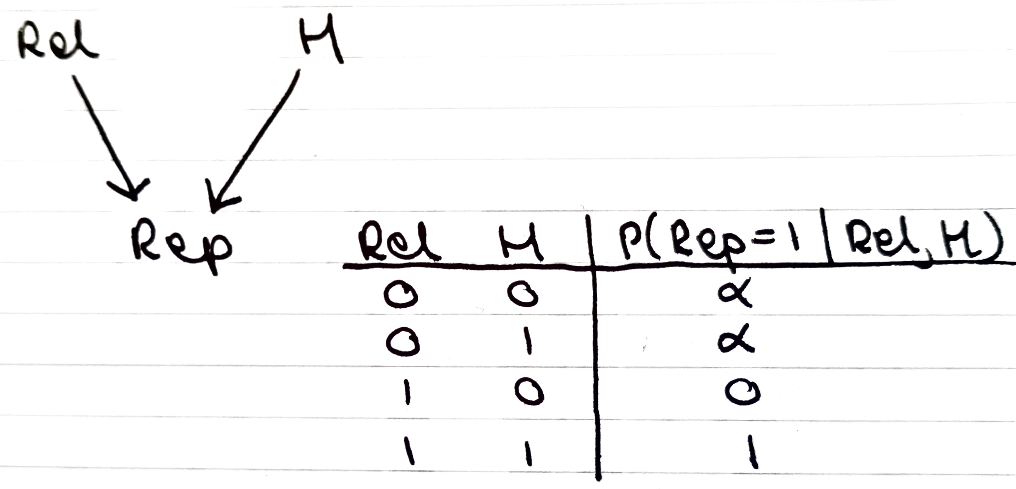
Bayseian network for Bovens and Hartmann model
\(\alpha\) is a parameter determining the probability of an unreliable source saying \(H\) is true (note that \(rep\) is independent of \(H\) in this case)
Probability of \(H\) is updated according to the report received and the prior probabilities: \(P'(H) = P(H \mid rep)\) (I think…)
Olsson model:
Also considers anti-reliability: sources who consistently lie
Focal agent maintains and updates a reliability distribution \(\tau\)
I think this is a random variable which gives the reliability of the source providing the information. Its variance decreases over time as our agent’s view of the source becomes more certain over time; its mean goes up or down depending on how the source’s claims relate to our agent’s beliefs
Presumable \(\tau\) takes values in something like \([-1, 1]\) to represent a range form anti-reliable to reliable. But the paper does not seems to make this explicit
Skimmed the rest: it gets really philosophical before going into some empirical analysis on simulated data
Algorithms for automatic ranking of participants and tasks in an anonymized contest (2017)
(Jiao, Yang and Ravi, R and Gatterbauer, Wolfgang)
Summary:
Introduces some new problems based on chain editing
Classifies their computational complexity
Background:
A set \(S\) of participants attempt a set of tasks \(Q\)
Each participant attempts all tasks but may only succeed at a subset
Aim to rank participants by their task-solving strength, and rank tasks by their difficulty
E.g. for MOOCs (massively open online courses) with crowdsourced questions which need to be graded automatically
Model:
Can be represented a bipartite graph \((S \cup Q, E)\) where \((s, q) \in E\) iff \(s\) succeeds at task \(q\).
\(n = |S| + |Q|\) is the parameter wrt which computation complexity is studied
Let \(N(x) = \{y : (x, y) \in E\}\) denote the neighbourhood of a node
\(s_1\) is stronger than \(s_2\) iff \(N(s_2) \supset N(s_1)\)
\(q_1\) is harder than \(q_2\) iff \(N(q_2) \subset N(q_1)\).
An ordering \(\succeq\) of the questions satisfies the interval property iff \(N(s)\) is an interval wrt \(\succeq\) for each \(s\) 2
An ordering \(\sqsupseteq\) of the participants satisfies the nesting property if \(s_1 \sqsupseteq s_2\) implies \(N(s_1) \supseteq N(s_2)\), i.e. if \(\sqsupseteq\) respects the ‘stronger-than’ ordering.
These are the ‘perfect-world’ situations where weak students are always worse than strong students, and easy questions are always answered correctly by more students.
Authors show that an interval ordering exists if and only if a nesting ordering exists. Moreover the interval ordering can be found from the nesting one (and vice versa) in polynomial time.
Problems:
Ideal Mutual Orderings (IMO): Find ordering of participants with the nesting property, or output NO if no such ordering exist
Can be solved in polynomial time
Chain Editing (CE): Find minimum set of edge edits (additions and deletions) so that IMO has a solution
Idea is that good students sometimes make mistakes, and poor students sometimes get lucky. A ‘close’ chain graph which admits a nested ordering is the best guess for the ‘true’ perfect-world performance of students
Chain Addition (CA): Same as CE but only additions are allowed
Models the situation where students can accidentally get questions wrong, but cannot accidentally get them right (e.g. numerical entry questions). In this case all edges are ‘true’ edges
Chain Deletion (CD): Same as CE but only deletions allowed
Similarly, this models a situation where students can accidentally get a question correct, but cannot accidentally get a question wrong.
CA and CD are ‘isomorphic’: solving one allows one to solve the other
Authors claim that a graph has a nested ordering if and only if its complement does
If we have an algorithm for CA and wish to solve CD for a graph \(G\), solve CA on the complement \(\bar{G}\). The edges \(F\) that need to be added to \(\bar{G}\) are the ones that need to be deleted from \(G\)
\(k\)-near variants:
Look at variations of CE, CA where an initial ordering of sources and questions is given, and sources/questions cannot be moved more than \(k\) positions from their original position in the ordering
Variations arise by allowing both orders to change or fixing one and finding a \(k\)-near ordering for the other, etc…
Main results:
Authors find polynomial time algorithms for some of the variants, and show that one is NP-hard
- 1
The main author’s PhD was sponsored by the US army, UK MoD and the ‘Petroleum Technology Development Fund’, which perhaps explains this particular focus.
- 2
\(X \subseteq Q\) is an interval iff for any \(x_1 \succeq x_2\) in \(X\) and any \(y \in Q\), \(x_1 \succeq y \succeq x_2\) implies \(y \in X\).